Survival Analysis: Telco Customer Churn — Report

Author: zhaozixi (12311625)
Date: April 2026
Approach: Hybrid PySpark + Lifelines (Kaplan-Meier, Cox PH, Log-Logistic AFT, CLV)

---

1. Data Preparation (Medallion Architecture)

Bronze Layer — Raw Ingestion

A SparkSession was initialized with 4 GB driver memory and Adaptive Query Execution enabled. The Telco Customer Churn dataset was ingested from a local CSV into the Bronze layer using an explicit StructType schema (21 fields, never inferSchema) to guarantee deterministic column types. Notable design choices:

• totalCharges is read as StringType() in Bronze because the raw CSV contains blank strings that would coerce to NaN under numeric inference.
• churnString (Yes/No) is retained as-is in Bronze to preserve the original format.

Bronze layer result: 7,043 records × 21 columns.

Silver Layer — Curation & Filtering

The Bronze data was transformed into the Silver layer through three operations:

1. totalCharges cleaning: Trimmed whitespace, replaced empty strings with NULL, and cast to DoubleType.
2. Churn label conversion: churnString (Yes/No) → churn (1.0 = churned, 0.0 = active), then churnString dropped.
3. Business-rule filtering:
   • Retained only Month-to-month contracts (highest churn-risk segment).
   • Retained only customers with Internet service (DSL or Fiber Optic).

Silver layer result:

Metric	Value
Total records	3,351
Churned (Event = 1)	1,556
Active (Censored = 0)	1,795
Churn rate	46.4%

The 46.4% churn rate confirms that month-to-month internet subscribers represent a high-risk population, making them an ideal cohort for survival analysis.

---

2. Kaplan-Meier Survival Analysis

The Silver DataFrame (3,351 rows) was converted to Pandas for lifelines modeling. The Kaplan-Meier (KM) estimator provides a non-parametric estimate of the survival function S(t) — the probability that a customer remains active beyond tenure t.

2.1 Population-Level Survival Curve

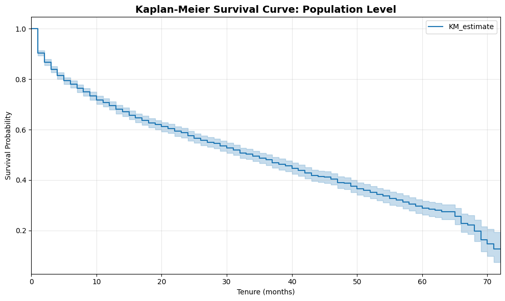
Median Survival Time: 34.0 months

This means a typical month-to-month internet customer has a 50% probability of remaining active for at least 34 months. The survival curve drops steeply in the first 6 months, then gradually flattens, indicating that the highest churn hazard occurs early in the customer lifecycle.

2.2 Survival by Gender

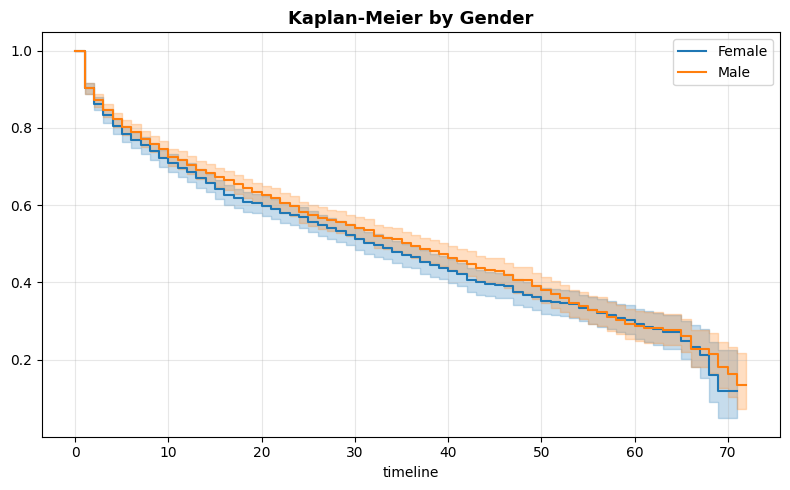
Log-rank test (Gender): test statistic = 2.039, p = 0.1533

The survival curves for Male and Female customers are nearly indistinguishable. The log-rank test fails to reject the null hypothesis (p > 0.05), confirming that gender is not a predictive factor for churn in this population.

2.3 Survival by Online Security

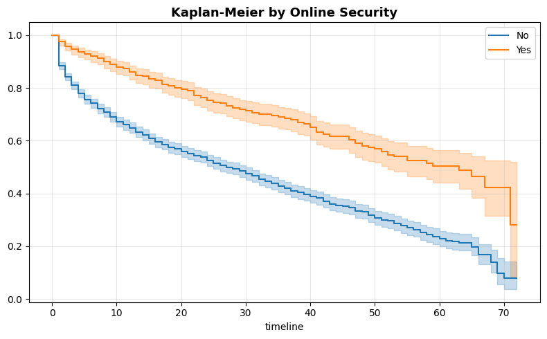
Log-rank test (Online Security): test statistic = 141.60, p = 1.19 × 10⁻³²

The divergence is dramatic. Customers with Online Security exhibit substantially higher survival probabilities across all tenure points. The extremely small p-value confirms that Online Security is a highly significant predictor of churn.

2.4 Survival Probabilities for DSL Customers (Months 0–9)

Month	Survival Probability
0	1.0000
1	0.9027
2	0.8644
3	0.8347
4	0.8105
5	0.7944
6	0.7839
7	0.7764
8	0.7685
9	0.7508

DSL customers lose approximately 25% of their base within the first 9 months, with the steepest decline occurring in months 1–2.

---

3. Cox Proportional Hazards Model

The Cox PH model quantifies the combined effect of multiple covariates on the instantaneous hazard of churning. Five variables were one-hot encoded and selected for modeling: dependents_Yes, internetService_DSL, onlineBackup_Yes, techSupport_Yes.

3.1 Model Summary

Modeling DataFrame: 3,351 rows × 6 columns
Events observed: 1,556 | Right-censored: 1,795

Covariate	coef	exp(coef) [HR]	HR Lower 95%	HR Upper 95%	z	p
dependents_Yes	−0.33	0.72	0.63	0.83	−4.64	< 0.005
internetService_DSL	−0.22	0.80	0.72	0.90	−3.68	< 0.005
onlineBackup_Yes	−0.78	0.46	0.41	0.52	−13.13	< 0.005
techSupport_Yes	−0.64	0.53	0.46	0.61	−8.48	< 0.005

Concordance = 0.64
Partial AIC = 22,639.90
Log-likelihood ratio test = 337.77 on 4 df (p < 10⁻⁷¹)

3.2 Hazard Ratio Interpretation

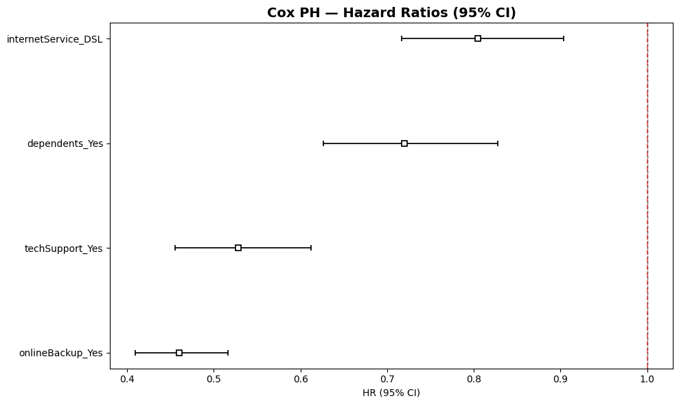
All four covariates have hazard ratios below 1.0, meaning they all reduce churn risk:

• onlineBackup_Yes (HR = 0.46): The strongest protective factor. Customers with Online Backup have a 54% lower instantaneous churn hazard compared to those without.
• techSupport_Yes (HR = 0.53): Customers with Tech Support have a 47% lower churn hazard.
• dependents_Yes (HR = 0.72): Customers with dependents have a 28% lower churn hazard, likely reflecting higher switching costs.
• internetService_DSL (HR = 0.80): DSL customers have a 20% lower churn hazard compared to Fiber Optic customers (the reference), suggesting Fiber Optic customers churn more readily — possibly due to higher expectations or competitive alternatives.

3.3 Proportional Hazards Assumption Test

The Cox PH model assumes hazard ratios remain constant over time. The check_assumptions() test was run using both Schoenfeld residuals (km and rank methods):

Covariate	Test	Test Statistic	p-value
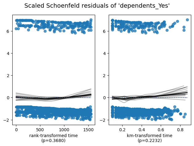
dependents_Yes	km	1.48	0.22
dependents_Yes	rank	0.81	0.37
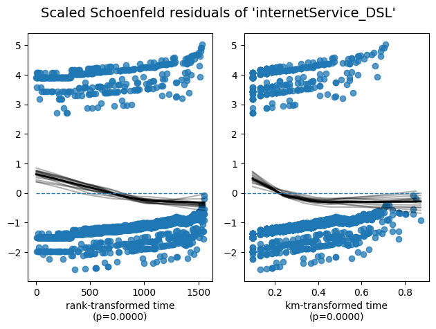
internetService_DSL	km	20.98	< 0.005 ❌
internetService_DSL	rank	26.71	< 0.005 ❌
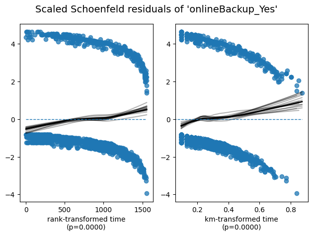
onlineBackup_Yes	km	17.80	< 0.005 ❌
onlineBackup_Yes	rank	17.47	< 0.005 ❌
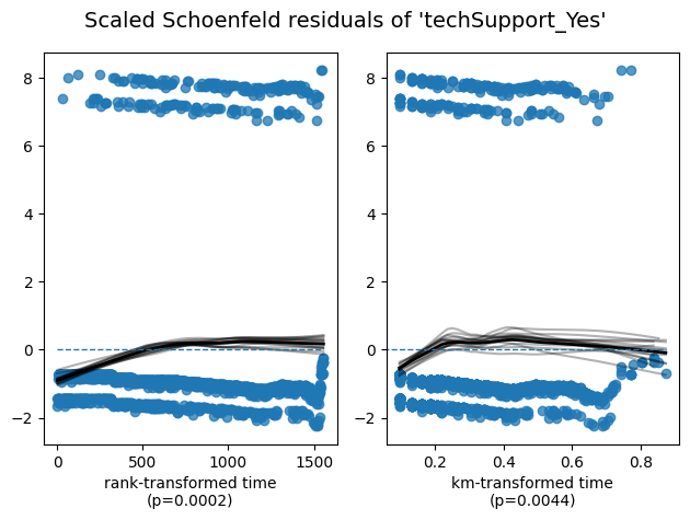
techSupport_Yes	km	8.09	< 0.005 ❌
techSupport_Yes	rank	13.76	< 0.005 ❌

Result: Three of four covariates (internetService_DSL, onlineBackup_Yes, techSupport_Yes) fail the proportional hazards test at p < 0.05. Only dependents_Yes passes. This means the hazard ratios for these variables are not constant over time, undermining the interpretability of the Cox PH coefficients.

3.4 Schoenfeld Residual Plots

The Schoenfeld residual plots visually confirm the violations:

• dependents_Yes: Flat lowess lines (p = 0.37 rank, p = 0.22 km) — PH assumption holds.
  

• internetService_DSL: Strongly non-flat lowess lines (p ≈ 0.00) — PH assumption violated.
  

• onlineBackup_Yes: Non-flat lowess lines (p ≈ 0.00) — PH assumption violated.
  

• techSupport_Yes: Non-flat lowess lines (p = 0.0002 rank, p = 0.0044 km) — PH assumption violated.
  

3.5 Log-Log KM Curve Verification

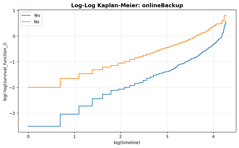
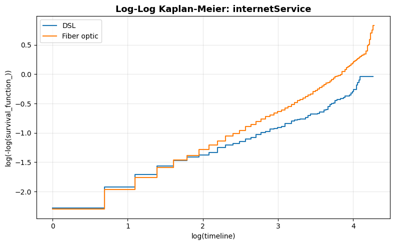
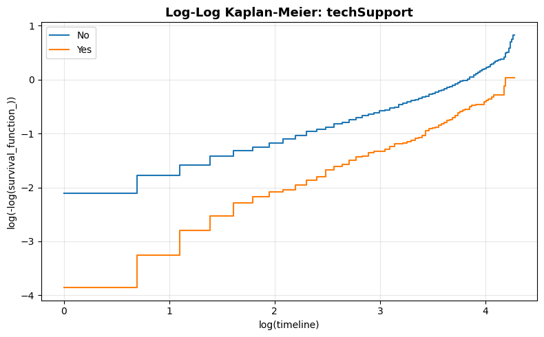
When the PH assumption holds, log-log KM curves should be parallel. All three plots show clearly non-parallel curves, visually confirming the statistical test results. The crossing and diverging patterns indicate that the effect of these covariates on churn hazard changes over time.

Implication: The Cox PH model's coefficients should be interpreted with caution. A parametric alternative (AFT model) that does not rely on the PH assumption is more appropriate for this dataset.

---

4. Accelerated Failure Time (AFT) Model

Given the PH violations in the Cox model, a Log-Logistic Accelerated Failure Time model was fitted. The AFT framework directly models survival time T rather than the hazard function, and does not require the proportional hazards assumption.

4.1 Feature Encoding

Eight categorical variables were one-hot encoded, and 10 predictor columns were selected: partner_Yes, multipleLines_Yes, internetService_DSL, onlineSecurity_Yes, onlineBackup_Yes, deviceProtection_Yes, techSupport_Yes, paymentMethod_Bank transfer (automatic), paymentMethod_Credit card (automatic).

AFT modeling DataFrame: 3,351 rows × 11 columns.

4.2 Model Summary

Median Survival Time: 135.51 months

Parameter	Covariate	coef	exp(coef)	coef Lower 95%	coef Upper 95%	z	p
α	deviceProtection_Yes	0.48	1.62	0.35	0.62	6.88	< 0.005
α	internetService_DSL	0.38	1.47	0.23	0.53	4.98	< 0.005
α	multipleLines_Yes	0.66	1.94	0.53	0.80	9.64	< 0.005
α	onlineBackup_Yes	0.81	2.25	0.68	0.95	11.63	< 0.005
α	onlineSecurity_Yes	0.86	2.37	0.69	1.03	10.12	< 0.005
α	partner_Yes	0.68	1.97	0.55	0.81	10.21	< 0.005
α	paymentMethod_Bank transfer (auto)	0.74	2.10	0.56	0.92	8.05	< 0.005
α	paymentMethod_Credit card (auto)	0.80	2.22	0.61	0.99	8.36	< 0.005
α	techSupport_Yes	0.69	1.99	0.52	0.86	7.90	< 0.005
α	Intercept (β₀)	1.59	4.91	1.46	1.72	24.47	< 0.005
β	Scale (σ)	0.12	1.13	0.08	0.16	5.71	< 0.005

Concordance = 0.73
AIC = 13,698.72
Log-likelihood ratio test = 877.49 on 9 df (p < 10⁻¹⁸²)

4.3 AFT Coefficient Interpretation

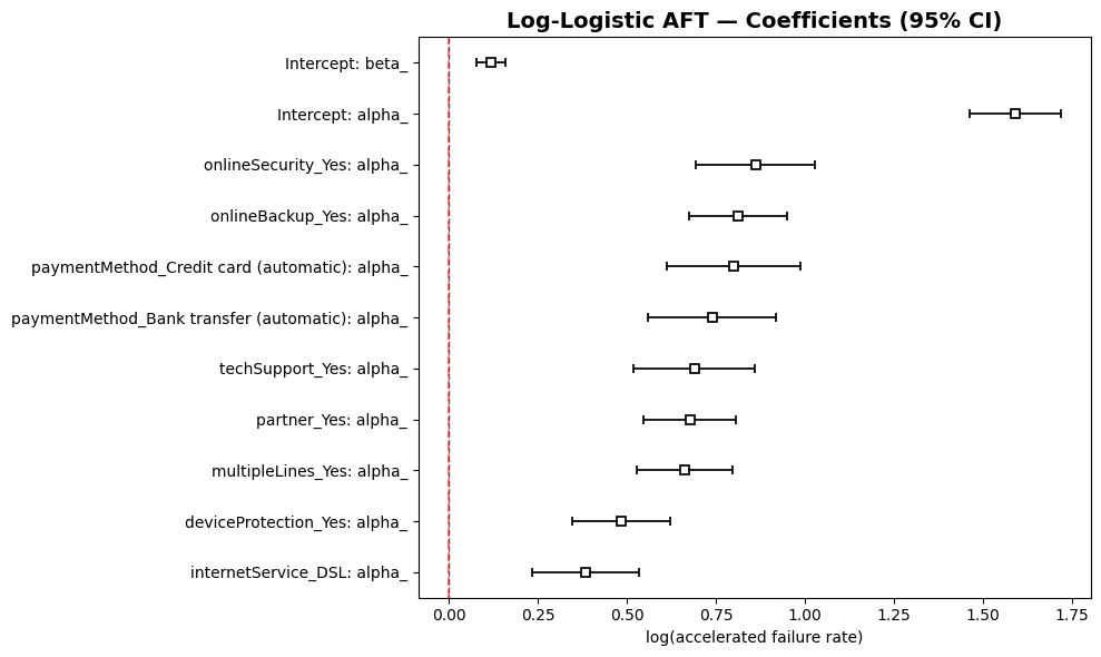
In the AFT framework, exp(coef) > 1 means the covariate accelerates time-to-churn (shortens expected tenure), while exp(coef) < 1 means it decelerates (lengthens tenure). Here, all α coefficients are positive, meaning all features in their encoded form accelerate churn relative to their respective reference categories.

Key interpretations (relative to reference groups):

• onlineSecurity_Yes (exp(coef) = 2.37): Customers with Online Security have an expected tenure 2.37× longer than those without. This is the largest protective effect.
• onlineBackup_Yes (exp(coef) = 2.25): Online Backup customers survive 2.25× longer.
• paymentMethod_Credit card (automatic) (exp(coef) = 2.22): Auto credit card payment is associated with 2.22× longer tenure vs. the reference (Electronic check).
• paymentMethod_Bank transfer (automatic) (exp(coef) = 2.10): Auto bank transfer yields 2.10× longer tenure.
• techSupport_Yes (exp(coef) = 1.99): Tech Support nearly doubles expected tenure.
• partner_Yes (exp(coef) = 1.97): Customers with partners survive 1.97× longer.
• multipleLines_Yes (exp(coef) = 1.94): Multiple Lines customers survive 1.94× longer.
• deviceProtection_Yes (exp(coef) = 1.62): Device Protection yields 1.62× longer tenure.
• internetService_DSL (exp(coef) = 1.47): DSL customers survive 1.47× longer than Fiber Optic customers.

Model parameters:

• Intercept (β₀) = 1.59 (exp = 4.91): The baseline scale factor for the log-logistic distribution.
• Scale (σ) = 0.12 (exp = 1.13): Controls the spread of the survival time distribution. A small σ indicates relatively tight clustering of survival times around the median.

4.4 Log-Odds KM Assumption Verification

For the Log-Logistic AFT model, the log-odds of the survival function should be approximately linear in log(time), and curves for different groups should be parallel (proportional odds assumption).

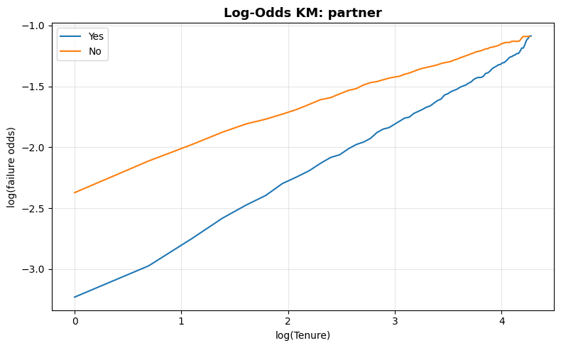
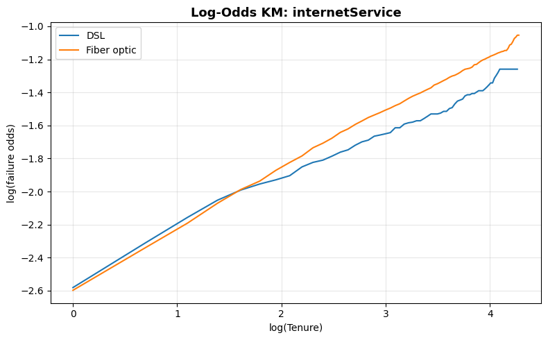
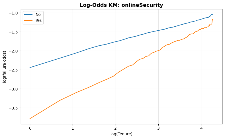
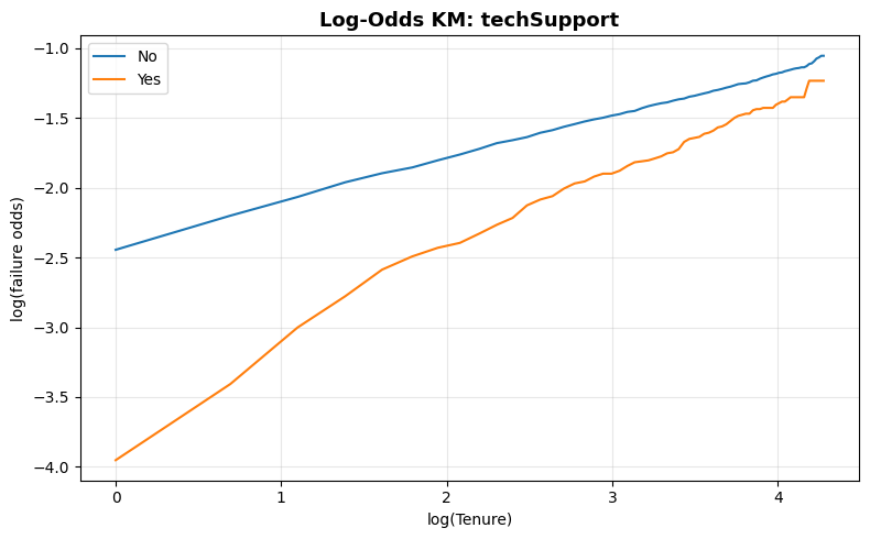
Assessment:

• Linearity: The curves are reasonably straight across most of the tenure range, confirming that the log-logistic distribution is an appropriate choice for modeling this data.
• Parallelism: The curves show moderate deviation from parallelism, particularly for internetService and techSupport at higher log-tenure values. This suggests the proportional odds assumption is approximately but not perfectly satisfied. However, the deviation is less severe than the PH violations in the Cox model, making the AFT model a more robust choice for this dataset.

4.5 Model Comparison: Cox PH vs. AFT

Metric	Cox PH	Log-Logistic AFT
Concordance	0.64	0.73
Assumption	PH violated (3/4 vars)	Proportional odds approximately satisfied
Parameters	4 covariates	10 covariates + scale

The AFT model achieves higher discriminative ability (Concordance 0.73 vs. 0.64) and operates under assumptions that are better satisfied by the data.

---

5. Customer Lifetime Value (CLV) Analysis

The Cox PH model's predict_survival_function() was used to compute month-by-month survival probabilities for a baseline customer profile (all covariates at reference values: no dependents, Fiber Optic, no Online Backup, no Tech Support). These probabilities were then translated into financial metrics.

5.1 CLV Calculation Framework

• Monthly Profit: $30.00 (fixed plan revenue assumption)
• Discount Rate: 10% annual IRR → 0.833% monthly
• Projection Horizon: 36 months

For each month t:

• Expected Monthly Profit = S(t) × $30
• NPV = Expected Monthly Profit / (1 + 0.00833)^t
• Cumulative NPV = Σ NPV up to month t

5.2 CLV Payback Table (Baseline Profile)

Month	Survival Prob.	Expected Monthly Profit	NPV	Cumulative NPV
1	0.8659	$25.98	$25.77	$25.77
2	0.8136	$24.41	$24.01	$49.78
3	0.7734	$23.20	$22.63	$72.41
4	0.7367	$22.10	$21.38	$93.79
5	0.7087	$21.26	$20.40	$114.19
6	0.6900	$20.70	$19.69	$133.88
7	0.6673	$20.02	$18.89	$152.77
8	0.6481	$19.44	$18.19	$170.96
9	0.6265	$18.79	$17.44	$188.40
10	0.6035	$18.10	$16.66	$205.06
11	0.5899	$17.70	$16.16	$221.22
12	0.5730	$17.19	$15.56	$236.78
13	0.5532	$16.60	$14.90	$251.68
14	0.5407	$16.22	$14.44	$266.12
15	0.5226	$15.68	$13.84	$279.96
16	0.5082	$15.25	$13.35	$293.31
17	0.4953	$14.86	$12.90	$306.21
18	0.4827	$14.48	$12.47	$318.68
19	0.4732	$14.20	$12.13	$330.81
20	0.4630	$13.89	$11.77	$342.58
21	0.4538	$13.61	$11.43	$354.01
22	0.4395	$13.19	$10.99	$365.00
23	0.4319	$12.96	$10.71	$375.71
24	0.4170	$12.51	$10.25	$385.96
25	0.4051	$12.15	$9.87	$395.83
26	0.3883	$11.65	$9.38	$405.21
27	0.3779	$11.34	$9.07	$414.28
28	0.3705	$11.12	$8.83	$423.11
29	0.3578	$10.73	$8.46	$431.57
30	0.3502	$10.51	$8.22	$439.79
31	0.3411	$10.23	$7.95	$447.74
32	0.3300	$9.90	$7.63	$455.37
33	0.3222	$9.67	$7.39	$462.76
34	0.3152	$9.46	$7.18	$469.94
35	0.3062	$9.19	$6.91	$476.85
36	0.2946	$8.84	$6.55	$483.40

(Note: Survival probability at month 36 = 0.2946, so the baseline customer has only a 29.5% chance of remaining active after 3 years.)

5.3 Cumulative NPV & Survival Visualization

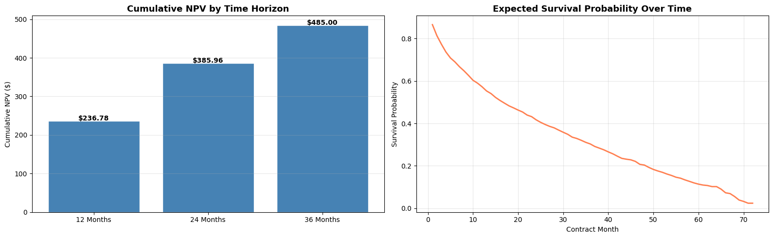
Key financial thresholds:

Horizon	Max Justifiable CAC
12 months	$236.78
24 months	$385.96
36 months	$483.40

The cumulative NPV represents the maximum customer acquisition cost (CAC) the company can incur without losing money. For the baseline customer profile:

• At 12 months, the break-even CAC is $236.78.
• At 24 months, it rises to $385.96.
• At 36 months, it reaches $483.40.

Any CAC above these thresholds would result in a negative return for the respective time horizon.

---

6. Conclusion & Business Recommendations

6.1 Summary of Findings

This analysis built an end-to-end survival analysis pipeline for telco customer churn, combining PySpark for industrial-scale data preparation (Bronze → Silver medallion architecture) and lifelines for statistical modeling.

Stage	Key Result
Data Preparation	7,043 → 3,351 records; 46.4% churn rate among month-to-month internet customers
Kaplan-Meier	Median survival: 34.0 months; Online Security is highly predictive (p < 10⁻³²), Gender is not (p = 0.15)
Cox PH Model	Concordance = 0.64; PH assumption violated for 3 of 4 covariates (DSL, Online Backup, Tech Support)
Log-Logistic AFT	Concordance = 0.73; Median survival = 135.51 months; All 10 covariates significant at p < 0.005
CLV (Baseline)	Max justifiable CAC: $236.78 (12mo), $385.96 (24mo), $483.40 (36mo)

6.2 Key Insights

1. Early churn is the dominant risk. The KM curve shows the steepest decline in the first 6 months. Survival probability drops from 100% to ~69% by month 6. This suggests that onboarding and early engagement are critical retention windows.

2. Service add-ons are the strongest retention drivers. Both the Cox PH and AFT models identify onlineSecurity and techSupport as the most powerful protective factors. In the AFT model, onlineSecurity_Yes extends expected tenure by a factor of 2.37× — the largest effect among all covariates.

3. Payment method matters. Automatic payment methods (bank transfer and credit card) are associated with 2.1× and 2.2× longer tenure, respectively. The convenience of auto-pay reduces involuntary churn and indicates higher customer commitment.

4. Fiber Optic customers are at higher risk. DSL customers consistently show lower churn than Fiber Optic customers across both models. This counterintuitive finding may reflect higher expectations among Fiber Optic users (who pay more) or greater availability of competitive alternatives.

5. The Cox PH model is inadequate for this data. The proportional hazards assumption is violated for most covariates, and the AFT model achieves superior discriminative ability (Concordance 0.73 vs. 0.64). The AFT model should be preferred for prediction and interpretation.

6.3 Actionable Recommendations

1. Invest in Tech Support and Online Security adoption. These two add-ons have the largest impact on extending customer lifetime. Consider bundling them at signup or offering free trials to new customers.

2. Target the first 6 months for retention interventions. With survival probability dropping to 69% by month 6, proactive outreach (e.g., satisfaction surveys, personalized offers) during this window could prevent the majority of churn events.

3. Promote automatic payment enrollment. Customers on auto-pay (bank transfer or credit card) survive 2× longer. Incentivize auto-pay signup during onboarding.

4. Investigate Fiber Optic churn drivers. The higher churn rate among Fiber Optic customers warrants qualitative research. Possible factors include service quality issues, price sensitivity, or competitor poaching.

5. Use AFT-based CLV to set CAC budgets. The $236.78 (12-month) and $385.96 (24-month) thresholds provide data-driven ceilings for customer acquisition spending. Profiles with protective features (e.g., Online Security + Tech Support) would have higher CLV, justifying proportionally higher CAC.

6. Consider time-varying Cox models or stratified models if the Cox PH framework is required (e.g., for regulatory reasons). Stratifying on internetService_DSL, onlineBackup_Yes, and techSupport_Yes would address the PH violations.